Chapter 6 Quantum perceptron

Figure 6.1: This section is a work in progress
The following chapter is an investigation into the quantum version of the classical perceptron algorithm, and is based on the previous works of (Kapoor, Wiebe, and Svore 2016)
The chapter is organized as follows: we first introduce the fundamentals of the classical version of the perceptron, then we present the online quantum perceptron algorithm and the version space quantum perceptron algorithm.
6.1 Classical perceptron
The perceptron is a machine learning algorithm that can be thought of as the most basic fundamental building block of more complex artificial neural networks (ANNs), or alternatively as a very simple form of neural network in and of itself.
The perceptron is a linear classifier used for binary predictions: its goal is to classify incoming data in one of two given categories. Like in any supervised learning tasks, the classifier is trained using a dataset of couples data points-labels and its goal is to generalize to previously unseen data points.
Unlike more complex learners, the textbook perceptron can only deal with linearly separable datasets. A dataset is said to be linearly separable if there exists at least one hyperplane that can successfully separate the elements of the dataset into distinct groups.
Two sets, \(\mathrm{A}\) and \(\mathrm{B}\), in an \(n-\)space are linearly separable only if there exists an \((n-1)\) hyperplane that shatters the two sets. In a 2-dimension space, the hyperplane is a line. In a 3D space it is a plane, and so on. (Note that in 2D, for instance, it could not be a curve! The linearity of this classifier make it so that you can only shatter the sets using hyperplanes. One could overcome this limitation by introducing kernels in the perceptron formulation or by projecting the data in a space, via “feature engineering”, so that they are linearly separable in the new space.)
Let us introduce the concept of linear separability using proper mathematical formalism.
Definition 6.1 (Linear Separability) Two sets \(\mathrm{A}\) and \(\mathrm{B}\) of points in an \(n\)-dimensional space are called absolutely linearly separable if \(n+1\) real numbers \(w_{1}\), \(\ldots\), \(w_{n}, b\) exist, such that every point \((x_{1}\), \(x_{2}\), \(\ldots\), \(x_{n})\) in \(\mathrm{A}\) satisfies : \[\begin{equation} \sum_{i=1}^{n} w_{i} x_{i}>b \end{equation}\] every point \(\mathrm{B}\) satisfies : \[\begin{equation} \sum_{i=1}^{n} w_{i} x_{i}<b \end{equation}\]
The general equation of the separation hyperplane would then be \(\sum_{i=1}^n w_ix_i + b = 0\).
The numbers \(w_i\) and \(b\) are often referred to as weights and bias respectively.
Without the bias term, the hyperplane that \(w\) defines would always have to go through the origin.
It is common practise to absorb \(b\) into the vector \(w\) by adding one additional constant dimension to the data points and the weigths vector.
In doing so, \({x}\) becomes
\([\begin{array}{c}{x}\\ 1\end{array}]\), and
\({w}\) becomes
\([\begin{array}{l}{w} \\ b\end{array}]\).
We can then verify that their inner product will yield,
\[\begin{equation}
\left[\begin{array}{c}
{x} \\
1
\end{array}\right]^{\top}\left[\begin{array}{l}
{w} \\
b
\end{array}\right]={w}^{\top} {x}+b
\end{equation}\]
From now on, we will write \(x\) and \(w\) assuming the bias is included in this way.
We will soon focus on how the perceptron learns the weights \(w_{i}\) and \(b\). However, assume for a while that the perceptron knows these numbers (i.e., it has been trained) and only needs to use them to classify the incoming data points in one of the two classes.
Given a data point \(x\), its coordinates \(x_{i}\) are weighted in a sum \(\sum w_{i} x_{i}\) and this result is passed to one “neuron” that has an activation function \(g\). The output of this activation function \(y=g(\sum w_{i} x_{i})\) is a binary value that represents one of the two possible classes. In general, the activation function can take many forms (ex: the sigmoid function, hyperbolic, step function, etc.) and return whichever couple of values (e.g., {0,1}, {-1,1}). For the remainder of this chapter, we will assume the sign function is used.
In other words, given a data point \(x\) and the weights \(w\), the perceptron classifies the point in the following way:
\[\begin{equation} y\left(x\right)=\operatorname{sign}\left({w}^{\top} {x}\right) \end{equation}\]
where \(y(x)=-1\) means that the sample belongs to one class and \(y(x)=+1\) means it belongs to the other, by a matter of convention.
The hyperplane identified by the weigths \(w\) is also called decision boundary as, using the sign activation function, the position of the data points w.r.t. it determines the output class.
6.1.1 Training the perceptron
In this book, we focus only on the online training algorithm, as this is handy for our quantum algorithms. We invite the interested reader to read more about the batch training.
The perceptron, like we should do, learns from its own errors but it also need somewhere to start from. Its training process happens in the following way. We initiate the perceptron with some random weights, feed it with many training couples data point-label, and let it shot its guess for each point. If the guess is correct, nothing happens. If the guess is wrong, the weights need to be updated.
Using the sign function, and considering a couple data point-label (\(x^{(i)}\), \(y^{(i)}\)) from the training set, the perceptron classifies the point correctly if \(y^{(i)}\left({w}^{\top} {x}^{(i)}\right)>0\) (this is because the class \(y^{(i)}\) has been encoded using values in \(\{-1,+1\}\)).
If a classification error is detected, the weights get modified by an amount that is proportional to the input \(x^{(i)}\). This process continues for a certain number of iterations, known as “epochs.” In the online learning regime, which is the one we investigate in this chapter, the update to the weight and bias vectors occurs for each and every misclassified data point iteratively throughout every epoch. During an epoch, each training data point is considered once. The training ends when there are no misclassified points in one epoch. We remind the reader that the training goal is to determine the weights that produce a linear decision boundary that correctly classifies the predictions.
The following pseudocode highlights the structure of the perceptron algorithm and identifies at which step in the processing schedule the error calculation and subsequent parametric updates occur.
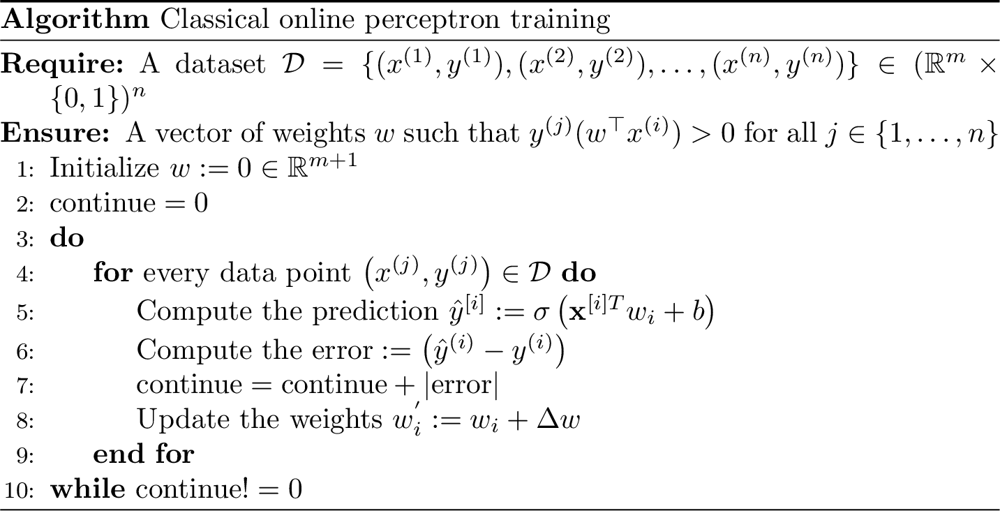
The update is computed by adding the amount \(\Delta w_{i}=\eta \cdot error \cdot x^{(i)}\) to the weights \(w\), where \(\eta\) is a learning rate end \(error = w^{\top}x-y^{(i)}\). Notice that if \(error\) and \(x^{(i)}_j\) have the same sign, the increment of \(w_j\) is positive (the strength increases) and otherwise decreases.
To sum up in an overall picture, the perceptron iteratively updates the linear boundary function (i.e., the hyperplane equation) that acts as the classifying condition between the two classes of the data, until no errors are detected and the algorithm converges. The training happens by minimizing the error on the training data set provided to the algorithm. Ultimately the identification of the weights allows for the distinction of data points belonging on one side of the boundary or the other.
Of course, if the data were not linearly separable, the training algorithm would run forever. The online training requires the existence of a margin between the two classes.
Definition 6.2 (Margin of a dataset) Let \(\{(x^{(1)}, y^{(1)}), (x^{(2)}, y^{(2)}), \dots, (x^{(n)}, y^{(n)})\}\) a dataset of \(n\) couples data points-labels, with \(x^{(i)} \in \mathbb{R}^m\) and \(y^{(i)} \in \{-1,+1\}\) for all \(i \in [n]\). We define the margin of this dataset as: \[\begin{equation} \gamma = \max_{q \in \mathbb{R}^{m}} \min_{i \in [n]} \frac{y^{(i)}q^{\top}x^{(i)}}{\|q\|\|x^{(i)}\|}. \end{equation}\]
It naturally follows that a dataset is linearly separable if and only if its margin is different from \(0\).
6.2 Online quantum perceptron
General Idea: Uses Grover’s search to more efficiently search for misclassified data points in the data set. This allows the perceptron algorithm to more quickly converge on a correct classifying hyperplane.
Where the quantum version of the online perceptron differs from that of its classical analogue is in how the data points are accessed for use within each individual epoch and in the number of times the perceptron needs to be used to classify the data points. In the classical version of the online perceptron, the training points are fed into the classification algorithm successively one by one, and a weight update is performed every time a point is misclassified. Imagine we have \(n\) data points and only the last ones of the epoch get misclassified: this requires \(O(n)\) evaluations of the classification function before the weights can be updated. The quantum version of the online perceptron deviates away from this mechanism of accessing the data points within an epoch in a "one at a time" fashion and lowers the number of time we need to call the classification function. The idea is to access the data points in superposition in a quantum state and apply the classification function to this state, so to apply the classification function linearly to all the data points at once, searching for the misclassified one.
Assume we have a dataset of \(\{x^{(1)}, \ldots, x^{(N)}\}\) vectors and \(\{y^{(1)}, \ldots, y^{(N)}\}\) labels. Without loss of generality, we assume that the training set consists of unit vectors and one-bit labels. Furthermore, we assume that the \(\{x^{(1)}, \ldots, x^{(N)}\}\) vectors can be classically represented using \(B\) bits. Then, with \(|x^{(1)}\rangle, \ldots, |x^{(n)}\rangle\) we denote the \((B+1)\)-bit representations of the data vectors, followed by the label bit. Note that each state \(|x^{(j)}\rangle\) corresponds to a state of the computational basis of the \((B+1)\)-dimensional Hilbert space.
Next, in order to construct our desired online quantum perceptron, we will need to have a mechanism with which to access the training data. We assume that the data is accessible via the following oracle \(U\).
\[\begin{align} U|j\rangle|{0}\rangle=|j\rangle|x^{(j)}\rangle\\ U^{\dagger}|j\rangle|{x^{(j)}}\rangle=|j\rangle|0\rangle \end{align}\]
As we discussed in previous chapters, because \(U\) and \(U^{\dagger}\) are linear operators, we have that \(U \frac{1}{\sqrt{n}}\sum_{j=1}^{n} |j\rangle|0\rangle=\frac{1}{\sqrt{n}}\sum_{j=1}^n |j\rangle|x^{(j)}\rangle\). A quantum computer can therefore access each training vector simultaneously using a single operation, while only requiring enough memory to store one of the \(|x^{(j)}\rangle\).
Next, we need a mechanism to test if a given weight configuration \(w\), correctly classifies a data point. First of all, we need to build a quantum circuit that implements the Boolean function \(f: \left(w,x^{(j)}, y^{(j)}\right) \mapsto \{0,1\}\), where \(f\left(w, x^{(j)}, y^{(j)}\right)\) is \(1\) if and only if the perceptron with weights \(w\) misclassifies the training sample \((x^{(j)}, y^{(j)})\). This circuit needs to adapt to the current weight configuration \(w\), which can be either “hardcoded” in the circuit (and the circuit would need to be updated everytime the vector changes) or be given as an input via use of extra qubits. Given access to such circuit, then we can define an operator, \(\mathcal{F_w}\): \[\begin{equation} \mathcal{F_w} |x^{(j)}\rangle=(-1)^{f(w, x^{(j)}, y^{(j)})} |x^{(j)}\rangle. \end{equation}\] \(\mathcal{F}_{w}\) is easily implemented on a quantum computer using a multiply controlled phase gate and a quantum implementation of the perceptron classification algorithm \(f_{w}\).
Now, we can use the unitary \(\mathcal{F}_{w}\) as an oracle for Grover’s algorithm (see Section 5.2). This allows for a quadratic reduction in the number of times that the training vectors need to be accessed by the classification function.
The following pseudocode sums up the online quantum perceptron algorithm.
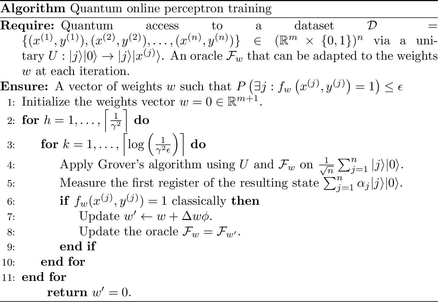
This algorithm gives birth to the following theorem, which formalizes the quadratic speedup.
Theorem 6.1 (Online quantum perceptron (Kapoor, Wiebe, and Svore 2016)) Given a training set that consists of unit vectors \(\{x^{(1)}, \ldots, x^{(n)}\}\) and labels \(\{y^{(1)}, \ldots, y^{(n)}\}\), with margin \(\gamma\), the number of applications of \(f\) needed to learn the weights \(w\) such that \(P\left(\exists j: f_{w}\left(x^{(j)}, y^{(j)}\right)=1\right) \leq \epsilon\) using a quantum computer is \(n_{\text {quant}}\) where \[\begin{equation} \Omega(\sqrt{n}) \ni n_{\text {quant}} \in O\left(\frac{\sqrt{n}}{\gamma^{2}} \log \left(\frac{1}{\epsilon \gamma^{2}}\right)\right) \end{equation}\] whereas the number of queries to \(f\) needed in the classical setting, \(n_{\text {class }}\), where the training vectors are found by sampling uniformly from the training data is bounded by \[\begin{equation} \Omega(n) \ni n_{\text {class}} \in O\left(\frac{n}{\gamma^{2}} \log \left(\frac{1}{\epsilon \gamma^{2}}\right)\right) . \end{equation}\]
Note that if the training data is supplied as a stream (as in the standard online model), then the upper bound for the classical model changes to \(n_{\text {class}} \in O\left(n / \gamma^{2}\right)\) because all \(n\) training vectors can be deterministically checked to see if they are correctly classified by the perceptron. A quantum advantage is therefore obtained if \(n \gg \log ^{2}\left(1 / \epsilon \gamma^{2}\right)\). (see (Kapoor, Wiebe, and Svore 2016) for a better explaination.)
Theorem 6.1 can easily be proved using Grover’s theorem (with exponential search, since we do not know the exact number of answers to the search problem. i.e., multiple data points can be misclassified) and two lemmas.
Lemma 6.1 Given only the ability to sample uniformly from the training vectors, the number of queries to \(f_{w}\) needed to find a training vector that the curnent perceptron model fails to classify correctly, or conclude that no such example exists, with probability \(1-\epsilon \gamma^{2}\) is at most \(O\left(n \log \left(1 / \epsilon \gamma^{2}\right)\right)\).
Lemma 6.2 Assuming that the training vectors \(\{x^{(1)}, \ldots, x^{(n)}\}\) are unit vectors and that they are drawn from two classes separated by a maryin of \(\gamma\) in feature space, the online quantum perceptron algorithm will either update the perceptron weights, or conclude that the current model provides a separating hyperplane between the two classes, using a number of queries to \(f_{w}\) that is bounded above by \(O\left(\sqrt{n} \log \left(1 / \epsilon \gamma^{2}\right)\right)\) with probability of failure at most \(\epsilon \gamma^{2}\).
The interested reader is encouraged consult the appendix of (Kapoor, Wiebe, and Svore 2016) for proofs of those lemmas. Furthermore, Novikoff’s theorem states that the \(1/\gamma^2\) is an upper bound in the number of times the algorithms described in these lemmas need to be applied, which is the reason for the first line of the algorithm and the \(1/\gamma^2\) term in the runtime.
6.3 Version space quantum perceptron
General idea: Discretize the space in which weight vectors live and use Grover’s search algorithm to find one vector that correctly classifies all the data points. Instead of searching among the data points, we are searching among weight vectors.
The key of the version space training algorithm is to search, among the possible weight vectors, one that correctly shatters the data points. Instead of iterating over the data points to update a weight vector, we will iterate over a discrete set of weight vectors to search a good one. The reason why this algorithm is called version space quantum perceptron lies in the space where the weight vector live, which is referred to as the version space.
Theorem 6.2 Given a training set with margin \(\gamma\), a weight vector \(w\) sampled from a spherical gaussian distribution \(\mathcal{N}(0,1)\) perfectly separates the data with probability \(\Theta(\gamma)\).
The main idea is to sample \(k\) sample hyperplanes \(w^{(1)}, \ldots, w^{(k)}\) from a spherical Gaussian distribution \(\mathcal{N}(0, \mathbb{1})\) such that \(k\) is large enough to guarantee us that there is at least one good weight vector. Theorem 6.2 tells us that the expected number of samples \(k\) scales as \(O(1/\gamma)\), and classically we would need to test all the \(n\) data points for at least \(O(1/\gamma)\) different vectors, with a cost \(\Omega(n/\gamma)\). By exploiting the power of Grover’s search we can have a quadratic speedup on \(k\) and achieve \(O(n/\sqrt{\gamma})\).
Like in the previous case, to use Grover, we need one unitary \(U\) that creates the weight vectors among which we search and one oracle \(\mathcal{F}\) that modifies the phase of the correct weight vectors.
The oracle \(U\) must do the following job: \[\begin{equation} U|j\rangle |0\rangle=|j\rangle |w^{(j)}\rangle \end{equation}\] for \(j \in \{1, \ldots, k\}\), giving access to the \(k\) sampled weight vectors. Clearly \(U\) is a linear operator and can be used with indexes in superposition, to give access to all the weight vectors simultaneously \(U\frac{1}{\sqrt{k}} \sum_{j=1}^{k} |j\rangle |0\rangle =\frac{1}{\sqrt{k}} \sum_{j=1}^{k} |j\rangle |w^{(j)}\rangle\).
On the other hand, the oracle \(\mathcal{F}\) should perform the following operation: \[\begin{equation} \mathcal{F}|w^{(j)}\rangle=(-1)^{1+\left(f\left(w^{(j)},x^{(1)}, y^{(1)}\right) \vee \cdots \vee f\left(w^{(j)},x^{(n)}, y^{(n)}\right)\right)}|w^{(j)}\rangle. \end{equation}\] Here \(f\left(w^{(j)}, x^{(i)}, y^{(i)}\right)\) works as in the quantum online perceptron algorithm: returns \(1\) if the data sample \((x^{(i)}, y^{(i)})\) is not correctly predicted by the weight \(w^{(j)}\). Basically, \(1+\left(f\left(w^{(j)},x^{(1)}, y^{(1)}\right) \vee \cdots \vee f\left(w^{(j)},x^{(n)}, y^{(n)}\right)\right)\) returns \(1\) if the vector \(w^{(j)}\) correctly classifies all the data points and \(0\) if there exists a training sample that is not correctly classified. Similarly to the previous case, this circuit can be built by “hardcoding” the knowledge of the data samples in each of the \(n\) functions or by creating one flexible function that accepts the vector and the points as input (by using additional qubits for the data points). This operation can be implemented with \(O(n)\) queries to \(f\).
Once we have the oracles \(U\) and \(\mathcal{F}\), we can sum up the algorithm in pseudocode.
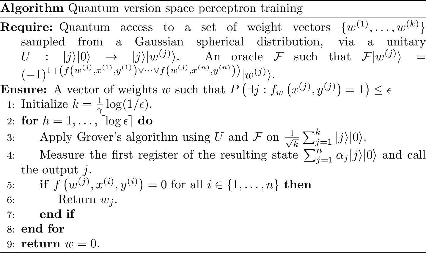
The following theorem formalizes the runtime of the algorithm.
Theorem 6.3 (Version space quantum perceptron (kapoor2016quantum)) Given a training set that consists of unit vectors \(x^{(1)}, \ldots, x^{(n)}\) and labels \(y^{(1)}, \ldots, y^{(n)}\), separated by a margin of \(\gamma\), the number of queries to \(f\) needed to infer a perceptron model \(w\), with probability at least \(1-\epsilon\), using a quantum computer is \(O\left(\frac{n}{\sqrt{\gamma}} \log \left(\frac{1}{\epsilon}\right)\right)\).
The proof of this theorem is straightforward from the statement of Grover’s algorithm and some statistics to bound the failure probability.