A Math and linear algebra
A.1 Norms, distances, trace, inequalities
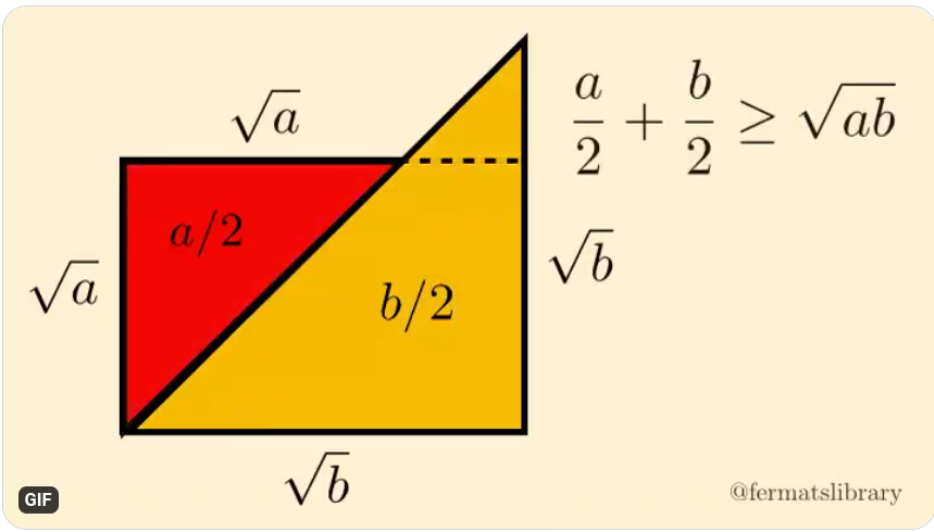
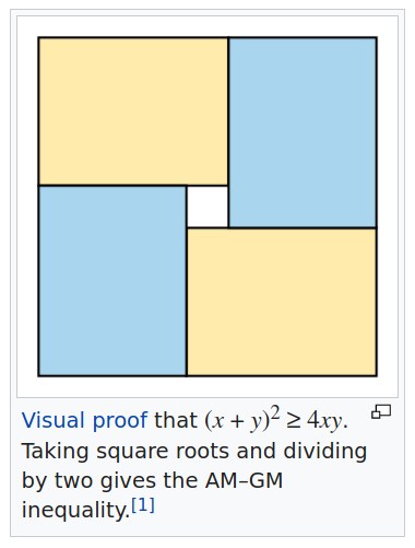
Take a look at this, and this.
Just remember that for a complez number \(z\), \(z\overline{z} = a^2 + b^2= |z|^2\), and \(\frac{1}{z} = \frac{\overline{z}}{\overline{z}z}\), and the conjugation is the mapping \(z = (a+ib) \mapsto \overline{z} = (a-ib)\).
Definition A.1 (Inner product) A function \(f: A \times B \mapsto \mathbb{C}\) is called an inner product \((a,b) \mapsto z\) if:
- \((a,b+c) = (a,b)+(a,c)\) (and respectively for \((a+c,b)\) )
- \((a,\alpha b) = \alpha (a,b)\)
Definition A.2 (Norm) A function \(f : \mathbb{R}^d \mapsto \mathbb{R}\) is called a norm if:
- \(\|x\| \geq 0 \forall x \in \mathbb{R}^{d}\), also \(\|x\|=0\) iff \(x=0\) (positive definiteness)
- \(\|\alpha x\| = \alpha \|x\| \forall x \in \mathbb{R}^{d}\) and \(\forall \alpha \in \mathbb{R}\) (positively homogeneous)
- \(\|x\|-\|y\| \leq \|x + y\| \leq \|x\| + \|y\|\) (triangle inequality).
Note that along with triangle inequality you might also need to know the reverse triangle inequality
The triangle inequality is basically the subadditivity property of the norm. It is simople to see that norms are not linear operators.
Theorem A.1 (Cauchy(-Bunyakovsky)-Schwarz) \[|(x,y)| \leq \|x\| \|y\|\]
Proof. Note that by taking the square on both sides we get: \((x,y)^2 \leq (x,x)(y,y)\). Substituting \((x,y)=\|x\| \|y\| cos(\theta)\), we get: \[|\|x\|^2\|y\|^2 cos^2(\theta) | \leq (x,x)(y,y)\] The inequality follows from noting that \(|cos(\theta)|\) is always \(\leq 1\).
Remark. It is simple to see - using Cauchy-Schwarz - that for a vector \(x\) we have that: \[\|x\|_1 \leq \sqrt{n} \|x\|_2 \]
We will use the following matrix norms:
- \(\|A\|_0\) as the number of non-zero elements of the matrix \(A\),
- \(\|A\|_1 = \max\limits_{1 \leq j \leq n} \sum_{i=0}^n |a_{ij}|\) is the maximum among the sum of the absolute value along the columns of the matrix,
- \(\|A\|_2 = \|A\| = \sigma_1\) is the biggest singular value of the matrix,
- \(\|A\|_\infty = \max\limits_{1 \leq i \leq m} \sum_{j=0}^n |a_{ij}|\) is the maximum among the sum of the absolute values along the rows of the matrix,
- \(\left\lVert A\right\rVert_{\max}\) is the maximal element of the matrix in absolute value.
- \(\left\lVert A\right\rVert_F\) is the Frobenius norm of the matrix, defined as \(\sqrt{\sum_{ij}a_{ij}^2}\)
Note that for symmetric matrices, \(\|A\|_\infty = \|A\|_1\).
Exercise A.1 (bound error on product of matrices) Suppose that \(\|A - \overline{A}\|_F \leq \epsilon \|A\|_F\). Bound \(\|A^TA - \overline{A}^T\overline{A}\|_F\)
Definition A.3 (Distance) A function \(f : \mathbb{R}^d \times \mathbb{R}^d \mapsto \mathbb{R}\) is called a distance if:
- \(d(x,y) \geq 0\)
- \(d(x,y) = 0\) iif \(x=y\)
- \(d(x,y)=d(y,x)\)
- \(d(x,z) \leq d(x,y) + d(y,z)\)
Definition A.4 (Convex and concave function) A function \(f\) defined on a convex vector space \(D\) is said to be concave if, \(\forall \lambda \in [0,1]\), and \(\forall x,y \in D\):
\[f\left( (1-\alpha)x + \alpha y \right) \geq (1-\alpha) f(x) + \alpha f(y)\] Conversely, a function \(f\) defined on a convex vector space \(D\) is said to be convex if, \(\forall \lambda \in [0,1]\), and \(\forall x,y \in D\): \[f\left( (1-\alpha)x + \alpha y \right) \leq (1-\alpha) f(x) + \alpha f(y)\]
A.1.0.1 Properties of the trace operator
- \(Tr[A+B] = Tr[A] + Tr[B]\)
- \(Tr[A\otimes B] = Tr[A]Tr[B]\)
- \(Tr_1[A\otimes B] = Tr[A]B\)
- \(Tr[|a\rangle\langle b|] = \langle a|b\rangle\)
- \(Tr[AB] = \langle A, B \rangle\)
where inner product between matrices is basically defined pointwise as \(\sum_{ij}a_{ij}b_{ij}\)
Exercise A.2 Can you show that the last identity is true?
A.1.0.2 Properties of tensor product
Given two liner maps \(V_1 : W_1 \mapsto V_1\) and \(V_2 : W_2 \mapsto V_2\) we define the tensor product as the linear map: \[V_1 \otimes V_2 : V_1 \otimes V_2 \mapsto W_1 \otimes W_2 \]
- \(\alpha v \otimes w = v \otimes \alpha w = \alpha(v \otimes w)\)
- \(( v_1 + v_2) \otimes w = (v_1 \otimes w) + (v_2 \otimes w)\) (and the symmetric of it)
- \(|\psi_1\rangle\langle\phi_1| \otimes |\psi_2\rangle\langle\phi_2| = |\psi_1\rangle|\psi_2\rangle \otimes \langle\phi_1|\langle\phi_2|\)
When a basis is decided for representing linear maps between vector spaces, the tensor product becomes the Kroeneker product.
A.2 Linear algebra
A.2.1 Eigenvalues, eigenvectors and eigendecomposition of a matrix
Real matrices are important tools in Machine Learning as they allow to comfortably represent data and describe the operations to perform during an algorithm. Eigenvectors and eigenvalues are fundamental linear algebra concepts that provide important information about a matrix.
Definition A.5 (Eigenvalues and Eigenvectors (Section 6.1 page 289 from (Strang 2016) )) Let \(A\) be a \(\mathbb{R}^{n\times n}\) square matrix, \(q \in \mathbb{R}^{n}\) a non-zero vector and \(\lambda\) a scalar. If the following equation is satisfied \[Aq = \lambda q,\] then \(q\) is said to be an eigenvector of matrix \(A\) and \(\lambda\) is its associated eigenvalue.
To have a geometric insight into what eigenvectors and eigenvalues are, we can think of any matrix as a linear transformation in the \(\mathbb{R}^n\) space. Under this light, we can say that the eigenvectors of a matrix are those vectors of the space that, after the transformation, lie on their original direction and only get their magnitude scaled by a certain factor: the eigenvalue.
The eigenvalues reveal interesting properties of a matrix. For example, the trace of a matrix (i.e. the sum of the element along the main diagonal of a square matrix) is the sum of its eigenvalues \[Tr[A] = \sum_i^{n}\lambda_i,\] and its determinant is equal to the product of the eigenvalues (Section 6.1 page 294 from (Strang 2016)) \[det(A) = \prod_i^{n}\lambda_i.\]
Moreover, a matrix \(A\) with eigenvalues \(\{\lambda_1, ..., \lambda_k\}\) has an inverse only if all the eigenvalues are not zero. The inverse has eigenvalues \(\{\frac{1}{\lambda_1}, ..., \frac{1}{\lambda_k}\}\).
Generally, one eigenvalue can be associated with multiple eigenvectors. There might be a set of vectors \(E(\lambda) \subseteq \mathbb{R}^n\) such that for all those vectors \(q \in E(\lambda): Aq = \lambda q\). That is why for each eigenvalue we talk about an eigenspace.
Definition A.6 (Eigenspace (Definition 7.1.5 page 108 (Manara, Perotti, and Scapellato 2007) )) Let \(A\) be a \(\mathbb{R}^{n\times n}\) square matrix and \(\lambda\) be an eigenvalue of \(A\). The eigenspace of \(A\) related to \(\lambda\) is the space defined over the set of vectors \(E(\lambda) = \{ x: Ax = \lambda x\}\).
For each eigenspace, through the Gram-Schmidt procedure, starting from linearly independent vectors it is possible to identify a set of orthogonal eigenvectors that constitute a basis for the space. The basis that spans the space where all the eigenvectors of a matrix lie is called eigenbasis.
Definition A.7 (Eigenbasis) A basis for the space where all the eigenvectors of a matrix lie is called eigenbasis.
An important result is that vectors in different eigenspaces are linearly independent.
Lemma A.1 (Linear independence of eigenvectors (Lemma 7.2.3 page 112 from (Manara, Perotti, and Scapellato 2007) )) The set of vectors obtained by the union of the bases of the eigenspaces of a matrix is linearly independent.
This means that if the sum of the dimensions of the eigenspaces \(\sum_i dim(E(\lambda_i))\) equals \(n\), it is possible to find \(n\) eigenvectors of \(A\) that form a basis for the \(\mathbb{R}^n\) space. If that is the case, each vector that lies in \(\mathbb{R}^n\) can be written as a linear combination of the eigenvectors of \(A\). Interestingly, matrices that have \(n\) linearly independent eigenvectors can be decomposed in terms of their eigenvalues and eigenvectors.
Theorem A.3 (Eigendecomposition or Diagonalization) Let \(A \in \mathbb{R}^{n \times n}\) be a square matrix with \(n\) linearly independent eigenvectors. Then, it is possible to decompose the matrix as \[A = Q\Lambda Q^{-1}.\] Where \(Q \in \mathbb{R}^{n\times n}\) is an square matrix and \(\Lambda \in \mathbb{R}^{n\times n}\) is a diagonal matrix. In particular, each \(i^{th}\) column of \(Q\) is an eigenvector of \(A\) and the \(i^{th}\) entry of \(\Lambda\) is its associated eigenvalue.
The matrices that can be eigendecomposed are also said diagonalizable, as in practice the theorem above states that such matrices are similar to diagonal matrices. Unfortunately, not all the square matrices have enough independent eigenvectors to be diagonalized. The Spectral Theorem provides us with a set of matrices that can always be eigendecomposed.
Theorem A.4 (Spectral theorem) Every symmetric matrix is diagonalizable \(A = Q\Lambda Q^{-1}\). Furthermore, its eigenvalues are real and it is possible to choose the columns of \(Q\) so that it is an orthogonal matrix.
Recall that a matrix \(Q\) is said to be orthogonal if \(QQ^T=Q^TQ = \mathbb{I}\), therefore \(Q^{-1} = Q^T\). The Spectral theorem, together with the fact that matrices like \(A^TA\) and \(AA^T\) are symmetric, will come in handy in later discussions.
Being able to eigendecompose a matrix allows performing some computations faster than otherwise. Some examples of operations that gain speed-ups from the eigendecomposed representation are matrix inversion and matrix exponentiation. Indeed, if we have a matrix \(A=Q\Lambda Q^{-1}\) its inverse can be computed as \(A^{-1}=Q\Lambda^{-1}Q^{-1}\) where \(\Lambda^{-1} = diag([\frac{1}{\lambda_1}, ... \frac{1}{\lambda_n}])\). It is easy to check that this matrix is the inverse of \(A\): \[AA^{-1} = (Q\Lambda Q^{-1})(Q\Lambda^{-1}Q^{-1}) = Q\Lambda\Lambda^{-1}Q^{-1} = QQ^{-1} = \mathbb{I}\] \[A^{-1}A = (Q\Lambda^{-1}Q^{-1})(Q\Lambda Q^{-1}) = Q\Lambda^{-1}\Lambda Q^{-1} = QQ^{-1} = \mathbb{I}.\] At the same time, the eigendecomposition of a matrix allows performing matrix exponentiation much faster than through the usual matrix multiplication. In fact, it is true that \(A^p = Q\Lambda^pQ^{-1}\). For instance, \[A^3 = (Q\Lambda Q^{-1})(Q\Lambda Q^{-1})(Q\Lambda Q^{-1}) = Q\Lambda(Q^{-1}Q)\Lambda(Q^{-1}Q)\Lambda Q^{-1} = Q\Lambda\Lambda\Lambda Q^{-1} = Q\Lambda^3Q^{-1}.\] Computing big matrix powers such as \(A^{100}\), with its eigendecomposed representation, only takes two matrix multiplications instead of a hundred.
Traditionally, the computational effort of performing the eigendecomposition of a \(\mathbb{R}^{n \times n}\) matrix is in the order of \(O(n^3)\) and may become prohibitive for large matrices (Partridge and Calvo 1997).
A.2.2 Singular value decomposition
Eigenvalues and eigenvectors can be computed only on square matrices. Moreover, not all matrices can be eigendecomposed. For this reason, we introduce the concepts of singular values and singular vectors, that are closely related to the ones of eigenvalues and eigenvectors, and offer a decomposition for all the kind of matrices.
Theorem A.5 (Singular Value Decomposition (Sections 7.1, 7.2 from [@linearalgebragilbert])) Any matrix \(A \in \mathbb{R}^{n \times n}\) can be decomposed as \[A = U\Sigma V^T\] where \(U \in \mathbb{R}^{n\times r}\) and \(V \in \mathbb{R}^{m\times r}\) are orthogonal matrices and \(\Sigma \in \mathbb{R}^{r\times r}\) is a diagonal matrix. In particular, each \(i^{th}\) column of \(U\) and \(V\) are respectively called left and right singular vectors of \(A\) and the \(i^{th}\) entry of \(\Sigma\) is their associated singular value. Furthermore, \(r\) is a natural number smaller then \(m\) and \(n\).
Another (equivaloent) definition of SVD is the following: \[A=(U, U_0)\begin{pmatrix} \Sigma & 0 \\ 0 & 0 \end{pmatrix} (V, V_0)^T.\] The matrix \(\Sigma\) is a diagonal matrix with \(\Sigma_{ii}=\sigma_i\) being the singular values (which we assume to be sorted \(\sigma_1 \geq \dots \geq \sigma_n\)).
The matrices \((U, U_0)\) and \((V, V_0)\) are unitary matrices, which contain a basis for the column and the row space (respectively \(U\) and \(V\)) and the left null-space and right null-space (respectively \(U_0\) and \(V_0\)). Oftentimes, it is simpler to define the SVD of a matrix by simply discarding the left and right null spaces, as \(A=U\Sigma V^T\), where \(U,V\) are orthogonal matrices and \(\Sigma \in \mathbb{R}^{r \times r}\) is a diagonal matrix with real elements, as we did in Theorem A.5.
Similarly to how eigenvalues and eigenvectors have been defined previously, for each pair of left-right singular vector, and the associated singular value, the following equation stands: \[Av = \sigma u.\]
If we consider the Singular Value Decomposition (SVD) under a geometric perspective, we can see any linear transformation as the result of a rotation, a scaling, and another rotation. Indeed, if we compute the product between a matrix \(A \in \mathbb{R}^{n\times m}\) and a vector \(x \in \mathbb{R}^m\) \[Ax = U\Sigma V^Tx = (U(\Sigma (V^Tx))).\] \(U\) and \(V^T\), being orthogonal matrices, only rotate the vector without changing its magnitude, while \(\Sigma\), being a diagonal matrix, alters its length.
It is interesting to note that the singular values of \(A\) - denoted as \(\{\sigma_1,..., \sigma_r\}\) - are the square roots \(\{\sqrt{\lambda_1},..., \sqrt{\lambda_r}\}\) of the eigenvalues of \(AA^T\) (or \(A^TA\)) and that the left and right singular vectors of \(A\) - denoted as \(\{u_1, ..., u_r\}\) and \(\{v_1, ..., v_r\}\) - are respectively the eigenvectors of \(AA^T\) and \(A^TA\).
The fact that each matrix can be decomposed in terms of its singular vectors and singular values, as in the theorem above, makes the relationship between singular values - singular vectors of a matrix and eigenvalues - eigenvectors of its products with the transpose clearer: \[AA^T = (U\Sigma V^T)(U\Sigma V^T)^T = U\Sigma V^TV\Sigma U^T = U\Sigma ^2U^T;\] \[A^TA = (U\Sigma V^T)^T(U\Sigma V^T) = V\Sigma U^TU\Sigma V^T = V\Sigma ^2V^T.\]
Note that the matrices \(AA^T\) and \(A^TA\) are symmetric matrices and so, for the Spectral theorem, we can always find an eigendecomposition. Moreover, note that they have positive eigenvalues: being the square roots of real positive eigenvalues, the singular values of a real matrix are always real positive numbers.
As the left and right singular vectors are eigenvectors of symmetric matrices, they can be chosen to be orthogonal as well. In particular, the left singular vectors of a matrix span the row space of the matrix, and the right singular vectors span the column space.
(#def:column_row_space) (Column (row) Space (Definition 8.1 page 192 [@schlesinger])) Let \(A\) be a \(\mathbb{R}^{n\times m}\) matrix. The column (row) space of \(A\) is the space spanned by the column (row) vectors of \(A\). Its dimension is equal to the number of linearly independent columns (rows) of \(A\).
The number \(r\) of singular values and singular vectors of a matrix is its rank.
Definition A.8 (Rank of a matrix (Definition 8.3, Proposition 8.4 page 193-194 from [@schlesinger]) ) The rank of a matrix is the number of linearly independent rows/columns of the matrix. If the matrix belongs to the \(\mathbb{R}^{n\times m}\) space, the rank is less or equal than \(min(n,m)\). A matrix is said to be full rank if its rank is equal to \(min(n,m)\).
The dimension of the null-space is the number of linearly-dependent columns. For a rank \(k\) matrix, the Moore-Penrose pseudo-inverse is defined as \(\sum_{i}^k \frac{1}{\sigma_i}u_i v_i^T\). Another relevant property of SVD is that the nonzero singular values and the corresponding singular vectors are the nonzero eigenvalues and eigenvectors of the matrix \(\begin{pmatrix} 0 & A \\ A^T & 0 \end{pmatrix}\):
\[ \begin{pmatrix} 0 & A \\ A^T & 0 \end{pmatrix} \begin{pmatrix} u_i \\ v_i \end{pmatrix} . = s_i \begin{pmatrix} u_i \\ v_i \end{pmatrix} \]
With \(s(A)\) or simply with \(s\) we denote the sparsity, that is, the maximum number of non-zero elements of the rows.
A.2.3 Singular vectors for data representation
Singular values and singular vectors provide important information about matrices and allow to speed up certain kind of calculations. Many data analysis algorithms, such as Principal Component Analysis, Correspondence Analysis, and Latent Semantic Analysis that will be further investigated in the following sections, are based on the singular value decomposition of a matrix.
To begin with, the SVD representation of a matrix allows us to better understand some matrix norms, like the spectral norm and the Frobenius norm (Strang 2016).
(#def:spectral_norm) (l2 (or Spectral) norm) Let \(A \in \mathbb{R}^{n\times m}\) be a matrix. The \(l_2\) norm of \(A\) is defined as \(\|A\|_2 = max_{x }\frac{\|A x \|}{\|x\|}\).
It is pretty easy to see that \(\|A\|_2 = \sigma_{max}\), where \(\sigma_{max}\) is the greatest singular value of \(A\). In particular, if we consider again the matrix \(A =U \Sigma V ^T\) as a linear transformation, we see that \(U\) and \(V ^T\) only rotate vectors \(||U x ||=||x ||\), \(||V x ||=||x ||\) while \(\Sigma\) changes their magnitude \(||\Sigma x || \leq \sigma_{max}||x ||\). For this reason, the \(l_2\) Norm of a matrix is also referred to as the Spectral Norm. During the rest of the work we will also use the notation \(||A ||\) to refer to the Spectral Norm.
Another important matrix norm that benefits from SVD is the Frobenius norm, defined in the following way.
Definition A.9 (Frobenius norm) Let \(A \in \mathbb{R}^{n\times m}\) be a matrix. The Frobenius norm of \(A\) is defined as \(\|A\|_F = \sqrt{\sum_i^n\sum_j^m a_{ij}^2}\).
It can be shown that also this norm is related to the singular values. ::: {.proposition} The Frobenius norm of a matrix \(A \in \mathbb{R}^{n\times m}\) is equal to the square root of the sum of squares of its singular values. \[\|A\|_F = \sqrt{\sum_i^r \sigma_{i}^2}\] :::
Proof. \[||A ||_F = \sqrt{\sum_i^n\sum_j^na_{ij}^2} = \sqrt{Tr[A A ^T]} = \sqrt{Tr[(U \Sigma V ^T)(U \Sigma V )^T]} =\] \[\sqrt{Tr[U \Sigma V ^TV \Sigma U ^T]} = \sqrt{Tr[U \Sigma \Sigma U ^T]} = \sqrt{Tr[U \Sigma ^2U ^T]} = \sqrt{\sum_{i=1}^{n}\sigma^2}\] From the cyclic property of the trace \(Tr[A B ] = Tr[B A ]\) it follows that \(Tr[U \Sigma ^2U ^T] = Tr[U ^TU \Sigma ^2] = Tr[\Sigma ^2]\), which is the sum of the squares of the singular values \(\sum_{i=1}^{n}\sigma^2\).
Another interesting result about the SVD of a matrix is known as the Eckart–Young–Mirsky theorem. ::: {.theorem #eckart-young-mirsky name=“Best F-Norm Low Rank Approximation”} Let \(A \in \mathbb{R}^{n \times m}\) be a matrix of rank \(r\) and singular value decomposition \(A = U \Sigma V ^T\). The matrix \(A ^{(k)} = U ^{(k)}\Sigma ^{(k)}V ^{(k)T}\) of rank \(k \leq r\), obtained by zeroing the smallest \(r-k\) singular values of \(A\), is the best rank-k approximation of \(A\). Equivalently, \(A _k = argmin_{B :rank(B )=k}(\|A - B \|_F)\). Furthermore, \(min_{B :rank(B )=k}(\|A - B \|_F) = \sqrt{\sum_{i=k+1}^r{\sigma_i}}\). :::
To get a clearer understanding of this result, we could rewrite \(A = U \Sigma V ^T = \sum_i^r\sigma_iu _iv _i^T\) and notice that matrix \(A\) is the sum of \(r\) matrices \(u _iv _i^T\) each scaled by a scalar \(\sigma_i\).
In practice, SVD decomposes matrix \(A\) in matrices of rank one, ordered by importance according to the magnitude of the singular values: the smaller the \(\sigma_i\), the smaller is the contribution that the rank-1 matrix gives to the reconstruction of \(A\). When the smallest singular values are set to 0, we still reconstruct a big part of the original matrix, and in practical cases, we will see that matrices can be approximated with a relatively small number of singular values.
Unfortunately though, calculating the singular vectors and singular values of a matrix is a computationally intensive task. Indeed, for a matrix \(A \in \mathbb{R}^{n\times m}\) the cost of the exact SVD is \(O\left( min(n^2m, nm^2) \right)\). Recently, there have been developed approximate methods that compute the Eckart-Young-Mirsky approximations of matrices in time \(O(knm)\), where k is the rank of the output matrix (Partridge and Calvo 1997), or in times that scale super-linearly on the desired rank and one dimension of the input matrix ??.
A.4 Inequalities
Theorem A.6 (Bernoulli inequalities)
Bernoulli inequality: for \(\forall n \in \mathbb{N}, x\geq -1\) \[(1+x)^n \geq 1+nx\] (Reader, check what happens if \(n\) even or odd!)
Generalized bernoully inequality: \(\forall r \in \mathbb{R} \geq 1\) or \(r \leq 0\), and \(x\geq -1\) \[(1+x)^r \geq 1+rx\]. For \(0 \leq r\leq 1\), \[(1+x)^r \leq 1+rx\]
Related inequality: for any \(x,r \in \mathbb{R}\), and \(r>0>\): \[(1+x)^r \leq e^{rx}\]
Theorem A.7 (Jensen inequality) Let \(X\) be a random variable with \(\mathbb{E}|X| \leq \infty\) and \(g : \mathbb{R}\to \mathbb{R}\) a real continious convex function. Then \[g(\mathbb{E}[X]) \leq \mathbb{E}[g(X)].\]
A mnemonic trick to remember the difference between convex and concave. ConvEX ends with EX, as the word EXponential, which is convex.
Theorem A.8 (Ljapunov's inequality) For any real \(0 \leq p \leq q\) and any real random variable, \(\|X\|_p \leq \|X\|_q\).
Theorem A.9 (Hölder's inequality) Let \(p,q>1\) that satisfy \(\frac{1}{p} + \frac{1}{q} = 1\). If \(\|X\|_p \leq \infty\) and \(\|X\|_q\) then \[\mathbb{E}[|XY|] \leq \|X\|_p \dot \|X\|_q.\]
Theorem A.10 (Minkowski's inequality) Let \(p>1\), \(\|X\|_p \leq \infty\) and \(\|Y\|_p \leq \infty\). Then: \[\|X+Y\|_p \leq \|X\|_p + \|Y\|_p.\]
A.5 Trigonometry
Always have in mind the following Taylor expansion:
Theorem A.11 (Taylor expansion of exponential function) \[e^{x} = \sum_{k=0}^\infty \frac{x^k}{k!}\] Note that this series is convergent for all \(x\)
From that, it is easy to derive that:
\[e^{\pm ix}= cos (x) \pm i sin(x) \]
Theorem A.12 (Nunzio's version of Euler's identity) For \(\tau = 2\pi\),
\[e^{i\tau} = 1 \]
Because of this, we can rewrite \(\sin\) and \(\cos\) as:
- \(\cos(x) = \frac{e^{ix} + e^{-ix}}{2}\)
- \(\sin(x)= \frac{e^{ix} - e^{-ix}}{2i}\)
Note that we can do a similar thing of A.11 for matrices. In this case, we define the exponential of a matrix via it’s Taylor expansion:
\[e^A = \sum_{k=0}^\infty \frac{A^k}{k!}\] The matrix exponential has the following nice properties (Walter 2018):
- \((e^A)^\dagger = e^{A^\dagger}\)
- \(e^{A\otimes I} = e^A \otimes I\)
- if \([A,B] = 0\), then \(e^Ae^B = e^{A+B}\).
- \(Ue^AU^\dagger = e^{UAU\dagger}\)
- \(det(e^A)= e^{Tr[A]}\)
A.5.0.1 Useful equalities in trigonometry
- \(\sin(a)\cos(b) = \frac{1}{2}(\sin(a+b)+\sin(a-b)) = 1/2(\sin(a+b)-\sin(b-a) )\)
- \(2 \cos x \cos y = \cos (x+y) + \cos (x-y)\)
Exercise A.3 Derive an expression for \(\cos(a+b)\).
Proof. Recall that \(e^{ix} = cos(x)+isin(x)\), \[e^{i(A+B)} = cos(a+b)+isin(a+b) = e^{iA}e^{iB} = (cos(a)+isin(a))(cos(b)+isin(b))\] \[cos(a+b)+isin(a+b) = cos(a)cos(b) + cos(a)+isin(b)+isin(a)cos(b) - sin(b)sin(a)\] \[cos(a+b)+isin(a+b) = cos(a)cos(b) + cos(a)isin(b)+isin(a)cos(b) - sin(b)sin(a)\] From this, it follows