Chapter 12 QML on real datasets
In this chapter, we discuss how to have a better idea on the performance of our algorithms on real dataset. This is very important, as the runtime of the algorithms we discuss here depends on the characteristics of the dataset, which might scale badly by increasing the size of the dataset. It’s our duty to see if this is the case. In the worst case, this might be due for each single dataset that we analyze. It this section we discuss two main approaches. We could either start by proving some properties of a dataset that we know is well-suitable to be analyzed by a certain algorithm. The idea is the following: if (quantum or classical) data analysis works well for a certain dataset, it might be because the algorithms that exploits certain structure in the dataset possess. We can exploit this intuition to prove some properties of the dataset that are expected to be analyzed by that algorithm. For example, this is the case for section 12.1.1, where we exploit the “cloud” structure of dataset that we often cluster using k-means (or q-means).
Secondly, we might just verify experimentally that the scaling of these parameters is favourable (they are small, they don’t grow by increasing the number of features and the number of samples, and so on..), and that the error introduced by the quantum procedures won’t perturb the quality of the data anaysis (in fact we will see that some noise might help regularizing the model, improving the classification accuracy).
12.1 Theoretical considerations
12.1.1 Modelling well-clusterable datasets
In this section, we define a model for the dataset in order to provide a tight analysis on the running time of our clustering algorithm. Thanks to this assumption, we can provide tighter bounds for its running time. Recall that for q-means we consider that the dataset \(V\) is normalized so that for all \(i \in [N]\), we have \(1 \leq \left\lVert v_{i}\right\rVert\), and we define the parameter \(\eta = \max_i{\left\lVert v_i\right\rVert^2}\). We will also assume that the number \(k\) is the “right” number of clusters, meaning that we assume each cluster has at least some \(\Omega(N/k)\) data points.
We now introduce the notion of a well-clusterable dataset. The definition aims to capture some properties that we can expect from datasets that can be clustered efficiently using a k-means algorithm. This notion of a well-clusterable dataset shares some similarity with the assumptions made in (Drineas, Kerenidis, and Raghavan 2002), but there are also some differences specific to the clustering problem.
Definition 12.1 (Well-clusterable dataset) A data matrix \(V \in \mathbb{R}^{n\times d}\) with rows \(v_{i} \in \mathbb{R}^{d}, i \in [n]\) is said to be well-clusterable if there exist constants \(\xi, \beta>0\), \(\lambda \in [0,1]\), \(\eta \leq 1\), and cluster centroids \(c_i\) for \(i\in [k]\) such that:
- (separation of cluster centroids): $d(c_i, c_j) i,j $
- (proximity to cluster centroid): At least \(\lambda n\) points \(v_i\) in the dataset satisfy \(d(v_i, c_{l(v_i)}) \leq \beta\) where \(c_{l(v_i)}\) is the centroid nearest to \(v_{i}\).
- (Intra-cluster smaller than inter-cluster square distances): The following inequality is satisfied \[4\sqrt{\eta} \sqrt{ \lambda \beta^{2} + (1-\lambda) 4\eta} \leq \xi^{2} - 2\sqrt{\eta} \beta.\]
Intuitively, the assumptions guarantee that most of the data can be easily assigned to one of \(k\) clusters, since these points are close to the centroids, and the centroids are sufficiently far from each other. The exact inequality comes from the error analysis, but in spirit it says that \(\xi^2\) should be bigger than a quantity that depends on \(\beta\) and the maximum norm \(\eta\).
We now show that a well-clusterable dataset has a good rank-\(k\) approximation where \(k\) is the number of clusters. This result will later be used for giving tight upper bounds on the running time of the quantum algorithm for well-clusterable datasets. As we said, one can easily construct such datasets by picking \(k\) well separated vectors to serve as cluster centers and then each point in the cluster is sampled from a Gaussian distribution with small variance centered on the centroid of the cluster.
Lemma 12.1 Let \(V_{k}\) be the optimal \(k\)-rank approximation for a well-clusterable data matrix \(V\), then \(\left\lVert V-V_{k}\right\rVert_{F}^2 \leq ( \lambda \beta^2 +(1-\lambda)4\eta)\left\lVert V\right\rVert^2_F\).
Proof. Let \(W \in \mathbb{R}^{n\times d}\) be the matrix with row \(w_{i} = c_{l(v_i)}\), where \(c_{l(v_i)}\) is the centroid closest to \(v_i\). The matrix \(W\) has rank at most \(k\) as it has exactly \(k\) distinct rows. As \(V_k\) is the optimal rank-\(k\) approximation to \(V\), we have \(\left\lVert V-V_{k}\right\rVert_{F}^{2} \leq \left\lVert V-W\right\rVert_F^2\). It therefore suffices to upper bound \(\left\lVert V-W\right\rVert_F^2\). Using the fact that \(V\) is well-clusterable, we have \[\left\lVert V-W\right\rVert_F^2 = \sum_{ij} (v_{ij} - w_{ij})^2 = \sum_{i} d(v_i, c_{l(v_i)})^2 \leq \lambda n \beta^2 + (1-\lambda)n4\eta,\] where we used Definition 12.1 to say that for a \(\lambda n\) fraction of the points \(d(v_i, c_{l(v_i)})^2 \leq \beta^{2}\) and for the remaining points \(d(v_i, c_{l(v_i)})^2 \leq 4\eta\). Also, as all \(v_{i}\) have norm at least \(1\) we have \(n \leq \left\lVert V\right\rVert_F\), implying that \(\left\lVert V-V_k\right\rVert^{2} \leq \left\lVert V-W\right\rVert_F^2 \leq ( \lambda \beta^2 +(1-\lambda)4\eta)\left\lVert V\right\rVert_F^2\).
The running time of the quantum linear algebra routines for the data matrix \(V\) in Theorem 5.11 depend on the parameters \(\mu(V)\) and \(\kappa(V)\). We establish bounds on both of these parameters using the fact that \(V\) is well-clusterable
Lemma 12.2 Let \(V\) be a well-clusterable data matrix, then \(\mu(V):= \frac{\left\lVert V\right\rVert_{F}}{\left\lVert V\right\rVert} = O(\sqrt{k})\).
Proof. We show that when we rescale \(V\) so that \(\left\lVert V\right\rVert = 1\), then we have \(\left\lVert V\right\rVert_{F}= O(\sqrt{k})\) for the rescaled matrix. From the triangle inequality we have that \(\left\lVert V\right\rVert_F \leq \left\lVert V-V_k\right\rVert_F + \left\lVert V_k\right\rVert_F\). Using the fact that \(\left\lVert V_k\right\rVert_F^2 = \sum_{i \in [k]} \sigma_i^2 \leq k\) and lemma 12.1, we have, \[\left\lVert V\right\rVert_F \leq \sqrt{ (\lambda\beta^2+(1-\lambda)4\eta)} \left\lVert V\right\rVert_F + \sqrt{k}\] Rearranging, we have that \(\left\lVert V\right\rVert_F \leq \frac{\sqrt{k}}{1-\sqrt{(\lambda\beta^2+(1-\lambda)4\eta)}} = O(\sqrt{k})\).
We next show that if we use a condition threshold \(\kappa_\tau(V)\) instead of the true condition number \(\kappa(V)\), that is we consider the matrix \(V_{\geq \tau} = \sum_{\sigma_{i} \geq \tau} \sigma_{i} u_{i} v_{i}^{T}\) by discarding the smaller singular values \(\sigma_{i} < \tau\), the resulting matrix remains close to the original one, i.e. we have that \(\left\lVert V - V_{\geq \tau}\right\rVert_F\) is bounded.
Lemma 12.3 Let \(V\) be a matrix with a rank-\(k\) approximation given by \(\left\lVert V- V_{k}\right\rVert_{F}\leq \epsilon' \left\lVert V\right\rVert_{F}\) and let \(\tau = \frac{\epsilon_{\tau}}{\sqrt{k}}\left\lVert V\right\rVert_F\), then \(\left\lVert V- V_{\geq \tau}\right\rVert_{F}\leq (\epsilon' + \epsilon_{\tau}) \left\lVert V\right\rVert_{F}\).
Proof. Let \(l\) be the smallest index such that \(\sigma_{l} \geq \tau\), so that we have \(\left\lVert V-V_{\geq \tau}\right\rVert_F = \left\lVert V-V_l\right\rVert_F\). We split the argument into two cases depending on whether \(l\) is smaller or greater than \(k\).
- If \(l \geq k\) then \(\left\lVert V-V_l\right\rVert_F \leq \left\lVert V-V_k\right\rVert_F \leq \epsilon' \left\lVert V\right\rVert_F\).
- If \(l < k\) then, \(\left\lVert V-V_l\right\rVert_F \leq \left\lVert V-V_k\right\rVert_F + \left\lVert V_k-V_l\right\rVert_F \leq \epsilon' \left\lVert V\right\rVert_F + \sqrt{\sum_{i=l+1}^k \sigma_i^2}\). As each \(\sigma_{i} < \tau\) and the sum is over at most \(k\) indices, we have the upper bound \((\epsilon' + \epsilon_{\tau}) \left\lVert V\right\rVert_F\).
The reason the notion of well-clusterable dataset was defined, was to be able to provide some strong guarantees for the clustering of most points in the dataset. Note that the clustering problem in the worst case is NP-hard and we only expect to have good results for datasets that have some good property. Intuitively, we should only expect \(k\)-means to work when the dataset can actually be clusterd in \(k\) clusters. We show next that for a well-clusterable dataset \(V\), there is a constant \(\delta\) that can be computed in terms of the parameters in Definition 12.1 such that the \(\delta\)-\(k\)-means clusters correctly most of the data points.
Lemma 12.4 Let \(V\) be a well-clusterable data matrix. Then, for at least \(\lambda n\) data points \(v_i\), we have \[\min_{j\neq \ell(i)}(d^2(v_i,c_j)-d^2(v_i,c_{\ell(i)}))\geq \xi^2 - 2\sqrt{\eta}\beta\] which implies that a \(\delta\)-\(k\)-means algorithm with any \(\delta < \xi^2 - 2\sqrt{\eta}\beta\) will cluster these points correctly.
Proof. By Definition 12.1, we know that for a well-clusterable dataset \(V\), we have that \(d(v_i, c_{l(v_i)}) \leq \beta\) for at least \(\lambda n\) data points and where \(c_{l(v_{i})}\) is the centroid closest to \(v_{i}\). Further, the distance between each pair of the \(k\) centroids satisfies the bounds \(2\sqrt{\eta} \geq d(c_i, c_j) \geq \xi\). By the triangle inequality, we have \(d(v_i,c_j) \geq d(c_j,c_{\ell(i)})-d(v_i,c_{\ell(i)})\). Squaring both sides of the inequality and rearranging, \[d^2(v_i,c_j) - d^2(v_i,c_{\ell(i)})\geq d^2(c_j,c_{\ell(i)}) - 2d(c_j,c_{\ell(i)})d(v_i,c_{\ell(i)}))\] Substituting the bounds on the distances implied by the well-clusterability assumption, we obtain \(d^2(v_i,c_j)-d^2(v_i,c_{\ell(i)}) \geq \xi^2 - 2\sqrt{\eta} \beta\). This implies that as long as we pick \(\delta < \xi^2 - 2\sqrt{\eta}\beta\), these points are assigned to the correct cluster, since all other centroids are more than \(\delta\) further away than the correct centroid.
12.2 Experiments
The experiments bypassed the construction of the quantum circuit and directly performed the noisy linear algebraic operations carried out by the quantum algorithm. The simulations are carried out on datasets that are considered the standard benchmark of new machine learning algorithms, inserting the same kind of errors that we expect to have in the real execution on the quantum hardware. In the experiments, we aim to study the robustness of data analysis to the noise introduced by the quantum algorithm, study the scaling of the runtime algorithm on real data and thus understand which datasets can be analyzed efficiently by quantum computers. The experiments are aimed at finding if the impact of noise in the quantum algorithms decreases significantly the accuracy in the data analysis, and if the impact of the error parameters in the runtime does prevent quantum speedups for large datasets.
12.2.1 Datasets
12.2.1.1 MNIST
MNIST (LeCun 1998) is probably the most used dataset in image classification. It is a collection of \(60000\) training plus \(10000\) testing images of \(28 \times 28 = 784\) pixels. Each image is a black and white handwritten digit between 0 and 9 and it is paired with a label that specifies the digit. Since the images are black and white, they are represented as arrays of 784 values that encode the lightness of each pixel. The dataset, excluding the labels, can be encoded in a matrix of size \(70000 \times 784\).
12.2.1.2 Fashon-MNIST
Fashion MNIST (Xiao, Rasul, and Vollgraf 2017) is a recent dataset for benchmarking in image classification. Like the MNIST, it is a collection of 70000 images composed of \(28 \times 28 = 784\) pixels. Each image represents a black and white fashion item among {T-shirt/top, Trouser, Pullover, Dress, Coat, Sandal, Shirt, Sneaker, Bag, Ankle boot}. Each image is paired with a label that specifies the item represented in the image. Since the images are black and white, they are represented as arrays of 784 values that encode the lightness of each pixel. The dataset, excluding the labels, can be encoded in a matrix of size \(70000 \times 784\).
12.2.1.3 CIFAR-10
CIFAR-10 (Krizhevsky et al. 2009) is another widely used dataset for benchmarking image classification. It contains \(60000\) colored images of \(32 \times 32\) pixel, with the values for each of the 3 RGB colors. Each image represents an object among {airplane, automobile, bird, cat, deer, dog, frog, horse, ship, truck} and is paired with the appropriate label. When the images are reshaped to unroll the three channels in a single vector, the resulting size of the dataset is \(60000 \times 3072\).
12.2.1.4 Research Paper
Research Paper (Harun-Ur-Rashid 2018) is a dataset for text classification, available on Kaggle. It contains 2507 titles of papers together with the labels of the venue where they have been published. The labels are {WWW, INFOCOM, ISCAS, SIGGRAPH, VLDB}. We pre-process the titles to compute a contingency table of \(papers \times words\): the value of the \(i^{th}-j^{th}\) cell is the number of times that the \(j^{th}\) word is contained in the \(i^{th}\) title. We remove the English stop-words, the words that appear in only one document, and the words that appear in more than half the documents. The result is a contingency table of size \(2507 \times 2010\).
12.2.2 q-means
12.2.2.1 MNIST pre-processing
From this raw data we first performed some dimensionality reduction processing, then we normalized the data such that the minimum norm is one. Note that, if we were doing \(q\)-means with a quantum computer, we could use efficient quantum procedures equivalent to Linear Discriminant Analysis, such as (Kerenidis and Luongo 2020), or other quantum dimensionality reduction algorithms like (Seth Lloyd, Mohseni, and Rebentrost 2014) (Cong and Duan 2015).
As preprocessing of the data, we first performed a Principal Component Analysis (PCA), retaining data projected in a subspace of dimension 40. After normalization, the value of \(\eta\) was 8.25 (maximum norm of 2.87), and the condition number was 4.53. Figure \(\ref{mnist-results-1}\) represents the evolution of the accuracy during the \(k\)-means and \(\delta\)-\(k\)-means for \(4\) different values of \(\delta\). In this numerical experiment, we can see that for values of the parameter \(\eta/\delta\) of order 20, both \(k\)-means and \(\delta\)-\(k\)-means reached a similar, yet low accuracy in the classification in the same number of steps. It is important to notice that the MNIST dataset, without other preprocessing than dimensionality reduction, is known not to be well-clusterable under the \(k\)-means algorithm.
| Algo | Dataset | ACC | HOM | COMP | V-M | AMI | ARI | RMSEC |
|---|---|---|---|---|---|---|---|---|
| k-means | Train | 0.582 | 0.488 | 0.523 | 0.505 | 0.389 | 0.488 | 0 |
| Test | 0.592 | 0.500 | 0.535 | 0.517 | 0.404 | 0.499 | - | |
| \(\delta\)-\(k\)-means, \(\delta=0.2\) | Train | 0.580 | 0.488 | 0.523 | 0.505 | 0.387 | 0.488 | 0.009 |
| Test | 0.591 | 0.499 | 0.535 | 0.516 | 0.404 | 0.498 | - | |
| \(\delta\)-\(k\)-means, \(\delta=0.3\) | Train | 0.577 | 0.481 | 0.517 | 0.498 | 0.379 | 0.481 | 0.019 |
| Test | 0.589 | 0.494 | 0.530 | 0.511 | 0.396 | 0.493 | - | |
| \(\delta\)-\(k\)-means, \(\delta=0.4\) | Train | 0.573 | 0.464 | 0.526 | 0.493 | 0.377 | 0.464 | 0.020 |
| Test | 0.585 | 0.492 | 0.527 | 0.509 | 0.394 | 0.491 | - | |
| \(\delta\)-\(k\)-means, \(\delta=0.5\) | Train | 0.573 | 0.459 | 0.522 | 0.488 | 0.371 | 0.459 | 0.034 |
| Test | 0.584 | 0.487 | 0.523 | 0.505 | 0.389 | 0.487 | - |
12.2.4 QEM
In this section, we discuss again Quantum Expectation-Maximization algorithm, and we present the results of some experiments on real datasets to estimate its runtime. We will also show some bound on the value of the parameters that governs it, like \(\kappa(\Sigma)\), \(\kappa(V)\), \(\mu(\Sigma)\), \(\mu(V)\), \(\delta_\theta\), and \(\delta_\mu\), and we give heuristic for dealing with the condition number. As we already have done, we can put a threshold on the condition number of the matrices \(\Sigma_j\), by discarding singular values which are smaller than a certain threshold. This might decrease the runtime of the algorithm without impacting its performances. This is indeed done often in classical machine learning models, since discarding the eigenvalues smaller than a certain threshold might even improve upon the metric under consideration (i.e. often the accuracy), by acting as a form of regularization (look at Section 6.5 of (Murphy 2012)). This in practice is equivalent to limiting the eccentricity of the Gaussians. We can do similar considerations for putting a threshold on the condition number of the dataset \(\kappa(V)\). Recall that the value of the condition number of the matrix \(V\) is approximately \(1/\min( \{\theta_1,\cdots, \theta_k\}\cup \{ d_{st}(\mathcal{N}(\mu_i, \Sigma_i), \mathcal{N}(\mu_j, \Sigma_j)) | i\neq j \in [k] \})\), where \(d_{st}\) is the statistical distance between two Gaussian distributions (Kalai, Moitra, and Valiant 2012). We have some choice in picking the definition for \(\mu\): in previous experiments it has been found that choosing the maximum \(\ell_1\) norm of the rows of \(V\) lead to values of \(\mu(V)\) around \(10\) for the MNIST dataset, as we saw on the experiments of QSFA, PCA and q-means. Because of the way \(\mu\) is defined, its value will not increase significantly as we add vectors to the training set. In case the matrix \(V\) can be clustered with high-enough accuracy by distance-based algorithms like k-means, it has been showed that the Frobenius norm of the matrix is proportional to \(\sqrt{k}\), that is, the rank of the matrix depends on the number of different classes contained in the data. Given that EM is just a more powerful extension of k-means, we can rely on similar observations too. Usually, the number of features \(d\) is much more than the number of components in the mixture, i.e. \(d \gg k\), so we expect \(d^2\) to dominate the \(k^{3.5}\) term in the cost needed to estimate the mixing weights, thus making \(T_\Sigma\) the leading term in the runtime. We expect this cost to be be mitigated by using \(\ell_\infty\) form of tomography but we defer further experiment for future research.
As we said, the quantum running time saves the factor that depends on the number of samples and introduces a number of other parameters. Using our experimental results we can see that when the number of samples is large enough one can expect the quantum running time to be faster than the classical one.
To estimate the runtime of the algorithm, we need to gauge the value of the parameters \(\delta_\mu\) and \(\delta_\theta\), such that they are small enough so that the likelihood is perturbed less than \(\epsilon_\tau\), but big enough to have a fast algorithm. We have reasons to believe that on well-clusterable data, the value of these parameters will be large enough, such as not to impact dramatically the runtime. A quantum version of k-means algorithm has already been simulated on the MNIST dataset under similar assumptions (Kerenidis et al. 2019). The experiment concluded that, for datasets that are expected to be clustered nicely by this kind of clustering algorithms, the value of the parameters \(\delta_\mu\) did not decrease by increasing the number of samples nor the number of features. There, the value of \(\delta_\mu\) (which in their case was called just \(\delta\)) has been kept between \(0.2\) and \(0.5\), while retaining a classification accuracy comparable to the classical k-means algorithm. We expect similar behaviour in the GMM case, namely that for large datasets the impact on the runtime of the errors \((\delta_\mu, \delta_\theta)\) does not cancel out the exponential gain in the dependence on the number of samples, and we discuss more about this in the next paragraph. The value of \(\epsilon_\tau\) is usually (for instance in scikit-learn (Pedregosa et al. 2011) ) chosen to be \(10^{-3}\). We will see that the value of \(\eta\) has always been 10 on average, with a maximum of 105 in the experiments.
12.2.5 QPCA
These experiment are extracted from (Bellante and Zanero 2022). This section shows several experiments on the MNIST, Fashion MNIST, CIFAR-10 and Research Papers datasets. In all the experiments, the datasets have been shifted to row mean \(0\) and normalized so that \(\sigma_{max} \leq 1\).
12.2.5.0.1 Explained variance distribution
First, we explore the distribution of the factor score ratios in the MNIST, Fashion MNIST, CIFAR-10 and Research Papers datasets, showing that a small number of singular values is indeed able to explain a great amount of the variance of the data. For all the four datasets, we compute the singular values and their factor score ratios and we plot them. The results of Figure 12.1 show a rapid decrease of the factor score ratios in all the datasets, confirming the expectations.
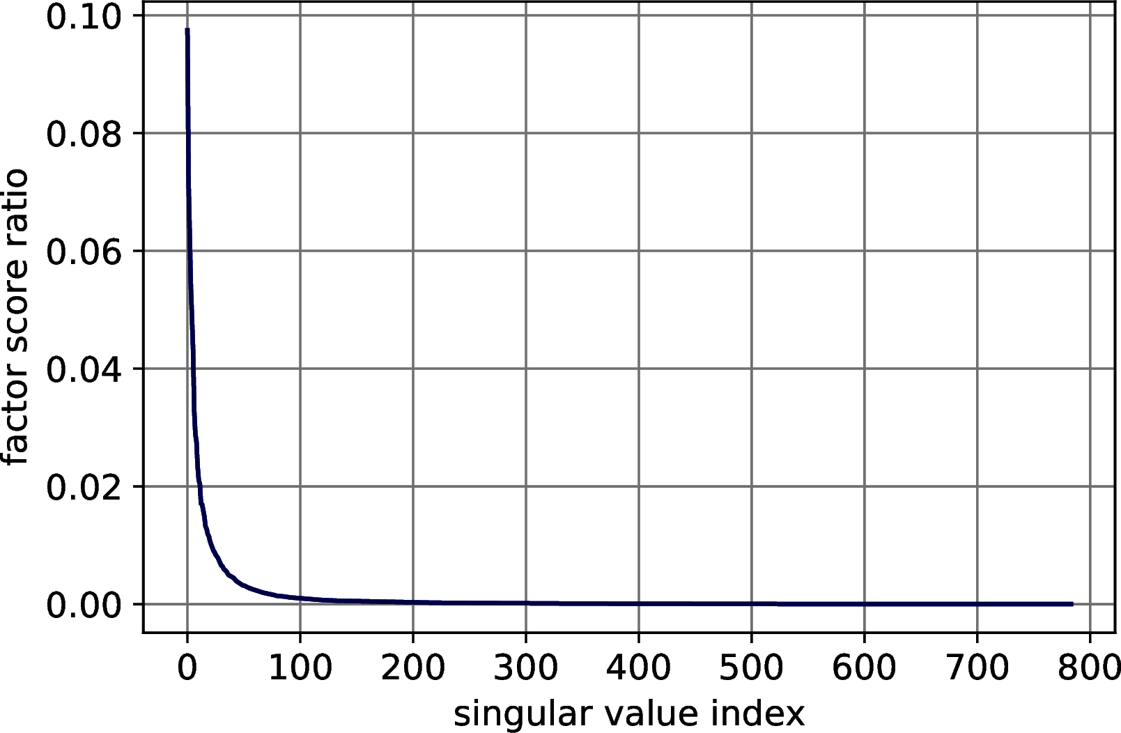
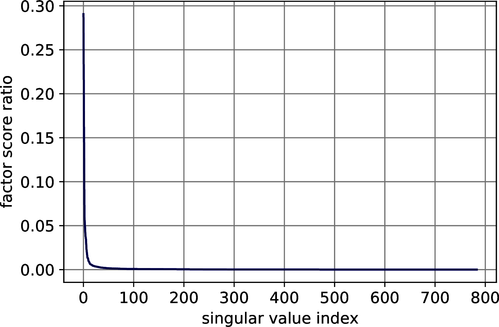
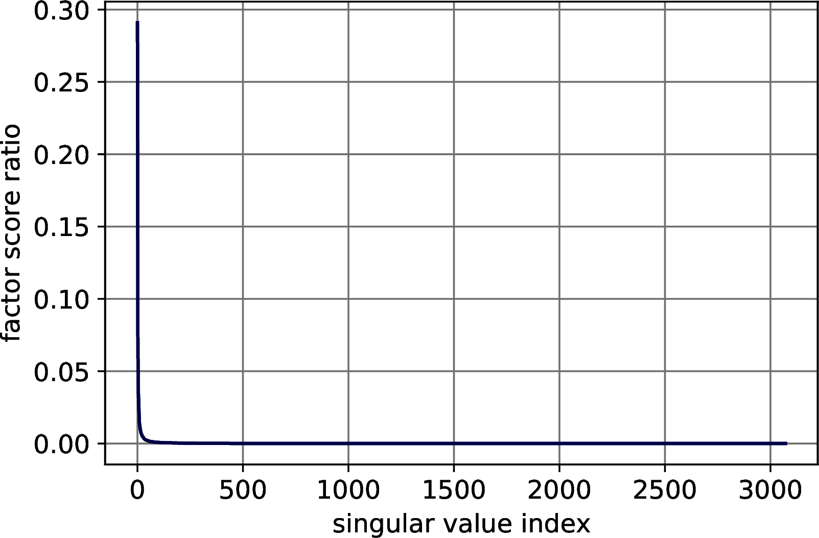
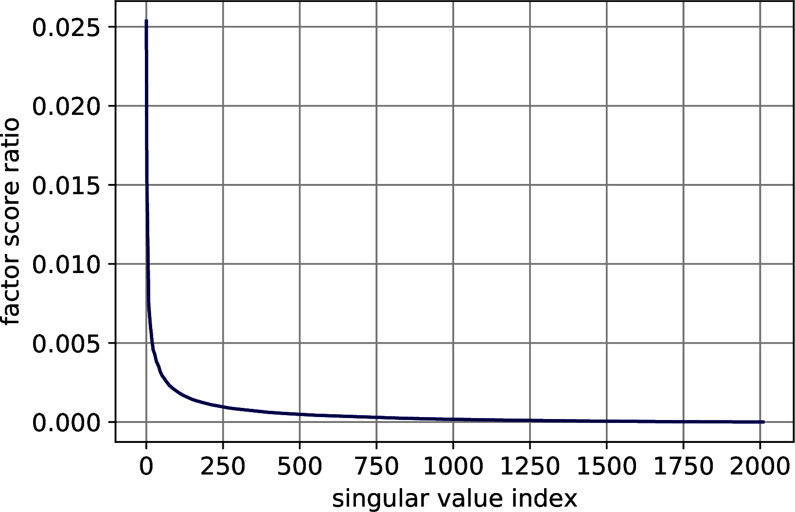
Figure 12.1: Explained variance distribution in datasets for machine learning. In order: MNIST, Fashion MNIST, CIFAR 10, Research Papers.
12.2.5.1 Image classification with quantum PCA
To provide the reader with a clearer view of the algorithms in Sections 7.2, 9.1.1 and their use in machine learning, we provide experiments on quantum PCA for image classification. We perform PCA on the three datasets for image classification (MNIST, Fashion MNIST and CIFAR 10) and classify them with a K-Nearest Neighbors. First, we simulate the extraction of the singular values and the percentage of variance explained by the principal components (top \(k\) factor score ratios’ sum) using the procedure from Theorem 7.3. Then, we study the error of the model extraction, using Lemma 9.1, by introducing errors on the Frobenius norm of the representation to see how this affects the accuracy.
12.2.5.1.1 Estimating the number of principal components
We simulate Theorem 7.3 to decide the number of principal components needed to retain 0.85 of the total variance. For each dataset, we classically compute the singular values with an exact classical algorithm and simulate the quantum state \(\frac{1}{\sqrt{\sum_j^r \sigma_j^2}} \sum_i^r \sigma_i|\sigma_i\rangle\) to emulate the measurement process. After initializing the random object with the correct probabilities, we measure it \(\frac{1}{\gamma^2} = 1000\) times and estimate the factor score ratios with a frequentist approach (i.e., dividing the number of measurements of each outcome by the total number of measurements). Measuring \(1000\) times guarantees us an error of at most \(\gamma=0.03\) on each factor score ratios. To determine the number of principal components to retain, we sum the factor score ratios until the percentage of explained variance becomes greater than \(0.85\). We report the results of this experiments in Table 12.2. We obtain good results for all the datasets, estimating no more than 3 extra principal components than needed.
| Parameter | MNIST | F-MNIST | CIFAR-10 |
|---|---|---|---|
| Estimated \(k\) | 62 | 45 | 55 |
| Exact \(k\) | 59 | 43 | 55 |
| Estimated \(p\) | 0.8510 | 0.8510 | 0.8510 |
| Exact \(p\) | 0.8580 | 0.8543 | 0.8514 |
| \(\gamma\) | 0.0316 | 0.0316 | 0.0316 |
The number of principal components can be further refined using Theorem 7.4. When we increase the percentage of variance to retain, the factor score ratios become smaller and the estimation worsens. When the factor score ratios become too small to perform efficient sampling, it is possible to establish the threshold \(\theta\) for the smaller singular value to retain using Theorems 7.4 and ??. If one is interested in refining the exact number \(k\) of principal components, rather than \(\theta\), it is possible to obtain it using a combination of the algorithms from Theorems 7.4, ?? and the quantum counting algorithm (Brassard et al. 2002) in time that scales with the square root of \(k\). Once that the number of principal components has been set, the next step is to use Theorem 7.5 to extract the top singular vectors. To do so, we can retrieve the threshold \(\theta\) from the previous step by checking the gap between the last singular value to retain and the first to exclude.
12.2.5.1.1.1 Studying the error in the data representation
We continue the experiment by checking how much error in the data representation a classifier can tolerate. We compute the exact PCA’s representation for the three datasets and a perform 10-fold Cross-validation error using a k-Nearest Neighbors with \(7\) neighbors. For each dataset we introduce error in the representation and check how the accuracy decreases. To simulate the error, we perturb the exact representation by adding truncated Gaussian error (zero mean and unit variance, truncated on the interval \([\frac{-\xi}{\sqrt{nm}},\frac{\xi}{\sqrt{nm}}]\)) to each component of the matrix. The graph in Figure @ref{fig:error-matrix} shows the distribution of the effective error on \(2000\) approximation of a matrix \(A\), such that \(\|A - \overline{A}\| \leq 0.1\). The distribution is still Gaussian, centered almost at the half of the bound.
Figure 12.2: Introducing some error in the Frobenius norm of a matrix \(A\). The error was introduced such that \(\|A - \overline{A}\| \leq 0.01\). The figure shows the distribution of the error over \(2000\) measurements.
The results show a reasonable tolerance of the errors, we report them in two set of figures. Figure 12.3 shows the drop of accuracy in classification as the error bound increases. Figure 12.4 shows the trend of the accuracy against the effective error of the approximation.
Figure 12.3: Classification accuracy of \(7\)-Nearest Neighbor on three machine learning datasets after PCA’s dimensionality reduction. The drop in accuracy is plotted with respect to the on the Frobenius norm of the difference between the exact data representation and its approximation. In order: MNIST, Fashion MNIST, CIFAR 10.
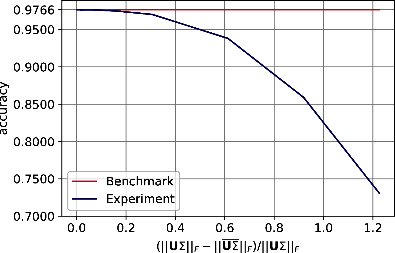

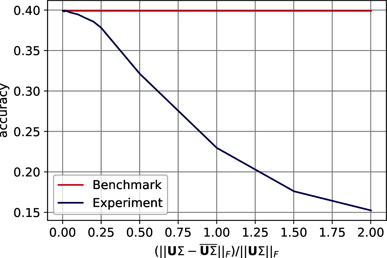
Figure 12.4: Classification accuracy of \(7\)-Nearest Neighbor on three machine learning datasets after PCA’s dimensionality reduction. The drop in accuracy is plotted with respect to the Frobenius norm of the difference between the exact data representation and its approximation. In order: MNIST, Fashion MNIST, CIFAR 10.
12.2.5.1.2 Analyzing the run-time parameters
As discussed in Section 9.1.1, the model extraction’s run-time is \(\widetilde{O}\left(\left( \frac{1}{\gamma^2} + \frac{kz}{\theta\sqrt{p}\delta^2}\right)\frac{\mu(A)}{\epsilon}\right)\), where \(A \in \mathbb{R}^{n\times m}\) is PCA’s input matrix, \(\mu(A)\) is a parameter bounded by \(\min(\|A\|_F, \|A\|_\infty)\), \(k\) is the number of principal components retained, \(\theta\) is the value of the last singular value retained, \(\gamma\) is the precision to estimate the factor score ratios, \(\epsilon\) bounds the absolute error on the estimation of the singular values, \(\delta\) bounds the \(\ell_2\) norm of the distance between the singular vectors and their approximation, and \(z\) is either \(n\), \(m\) depending on whether we extract the left singular vectors, to compute the classical representation, or the right ones, to retrieve the model and allow for further quantum/classical computation. This run-time can be further lowered using Theorem ?? if we are not interested in the factor score ratios. The aim of this paragraph is to show how to determine the run-time parameters for a specific dataset. We enrich the parameters of Table 12.2 with the ones in Table 12.3 and we discuss how to compute them. From the previous paragraphs it should be clear how to determine \(k\), \(\theta\), \(\gamma\) and \(p\), and it is worth noticing again that \(1/\sqrt{p} \simeq 1\). To bound \(\mu(A)\) we have computed \(\|A\|_F\) and \(\|A\|_\infty\). To compute the parameter \(\epsilon\) we have considered two situations: we need to allow for a correct ordering of the singular values; we need to allow for a correct thresholding. We refer to the first as the ordering \(\epsilon\) and to the second as the thresholding \(\epsilon\). To compute the first one it is sufficient to check the smallest gap between the first \(k\) singular values of the dataset. For the last one, one should check the difference between the last retained singular value and the first that is excluded. It follows that the thresholding \(\epsilon\) is always smaller than the ordering \(\epsilon\). For sake of completeness, we have run experiments to check how the Coupon Collector’s problem changes as \(\epsilon\) increases. Recall that in the proof of Theorem @ref(thm:top-k_sv_extraction) we use that \(\frac{1}{\sqrt{\sum_{i}^k \frac{\sigma_i^2}{\overline{\sigma}_i^2}}}\sum_i^k\frac{\sigma_i}{\overline{\sigma}_i} |u_i\rangle|v_i\rangle|\overline{\sigma}_i\rangle \sim \frac{1}{\sqrt{k}}\sum_i^k |u_i\rangle|v_i\rangle|\overline{\sigma}_i\rangle\) to say that the number of measurements needed to observe all the singular values is \(O(k\log(k))\), and this is true only if \(\epsilon\) is small enough to let the singular values distribute uniformly. We observe that the thresholding \(\epsilon\) always satisfy the Coupon Collector’s scaling, and we have plotted the results of our tests in Figure 12.5.
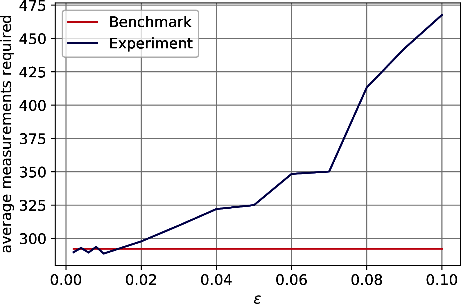
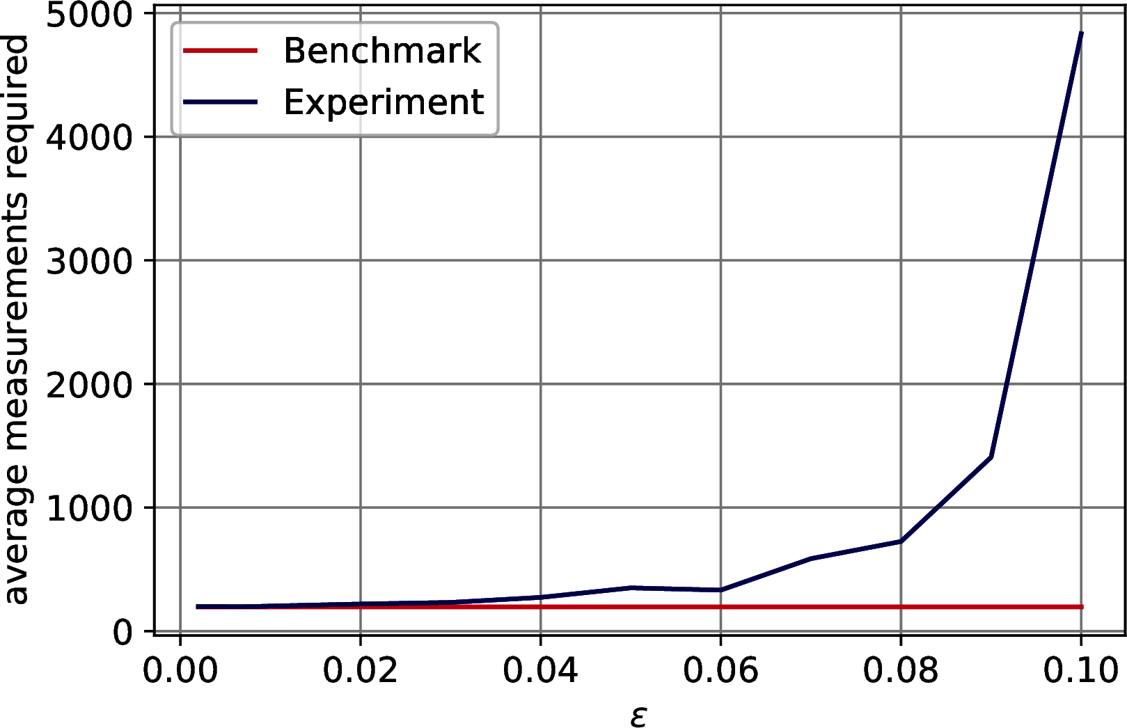
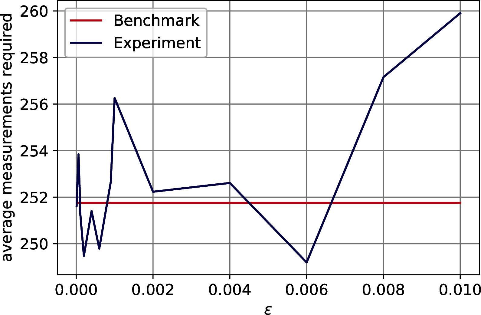
Figure 12.5: Number of measurements needed to obtain all the \(k\) singular values from the quantum state \(\frac{1}{\sqrt{\sum_i^r\sigma_i^2}}\sum_i^k \frac{\sigma_i}{\overline{\sigma}_i}|\overline{\sigma}_i\rangle\), where \(\|\sigma_i - \overline{\sigma}_i\| \leq \epsilon\), as \(\epsilon\) increases. The benchmark line is \(k\log_{2.4}(k)\). In order: MNIST, Fashion MNIST, CIFAR 10.
Furthermore, we have computed \(\delta\) by using the fact that \(\|A - \overline{A}\| \leq \sqrt{k}(\epsilon + \delta)\) (Lemma 9.1). By inverting the equation and considering the thresholding \(\epsilon\) we have computed an estimate for \(\delta\). In particular, we have fixed \(\|A - \overline{A}\|\) to the biggest value in our experiments so that the accuracy doesn’t drop more than \(1\%\).
Since we have considered the values of the effective errors instead of the bounds, our estimates are pessimistic.
| Parameter | MNIST | F-MNIST | CIFAR-10 |
|---|---|---|---|
| Ordr. \(\epsilon\) | 0.0003 | 0.0003 | 0.0002 |
| Thrs. \(\epsilon\) | 0.0030 | 0.0009 | 0.0006 |
| \(\|A\|_F\) | 3.2032 | 1.8551 | 1.8540 |
| \(\|A\|_\infty\) | 0.3730 | 0.3207 | 0.8710 |
| \(\theta\) | 0.1564 | 0.0776 | 0.0746 |
| \(\delta\) | 0.1124 | 0.0106 | 0.0340 |
These results show that Theorem 7.3, 7.4 and ?? can already provide speed-ups on datasets as small as the MNIST. Even though their speed-up is not exponential, they still run sub-linearly on the number of elements of the matrix even though all the elements are taken into account during the computation, offering a polynomial speed-up with respect to their traditional classical counterparts. On the other hand, Theorem 7.5 requires bigger datasets. On big low-rank datasets that maintain a good distribution of singular values, these algorithms are expected to show their full speed-up. As a final remark, note that the parameters have similar orders of magnitude.
12.2.5.1.3 Projecting the quantum data in the new quantum feature space
To end with, we have tested the value of \(\alpha\) (Definition 9.1, Lemma 9.3) for the MNIST dataset, fixing \(\varepsilon=0\) and trying \(p \in \{0.1,0.2,0.3,0.4,0.5,0.6,0.7,0.8,0.9\}\). We have observed that \(\alpha = 0.96 \pm 0.02\), confirming that the run-time of Corollary 9.1 can be assumed constant for the majority of the data points of a PCA-representable dataset.